Favourite Things

By Carl Goodwin in R

July 26, 2020

Each project closes with a table summarising the R tools used. By visualising the most frequently used packages and functions I can get a sense of where I may most benefit from going deeper into the latest package versions.

I may also spot superseded functions e.g. spread and gather improved by pivot_wider and pivot_longer. Or an opportunity to switch a non-tidyverse package for a newer tidyverse / tidymodels (or extension) alternative, e.g. the new tidyclust package brings cluster modelling to tidymodels and is used in Finding Happiness in ‘The Smoke’.

This page is regularly refreshed to incorporate new or modified projects; see the collapsed Details section at the foot of this page for the last modified date.

library(tidyverse)
library(tidytext)
library(rvest)
library(paletteer)
library(janitor)
library(glue)
library(kableExtra)
library(ggwordcloud)
library(fpp3)
library(tidymodels)
library(patchwork)

theme_set(theme_bw())

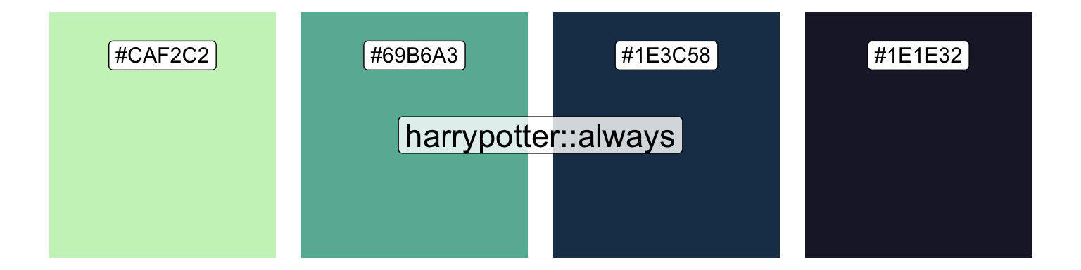
n <- 4
palette <- "harrypotter::always"

cols <- paletteer_c(palette, n = n)

tibble(x = 1:n, y = 1) |>
  ggplot(aes(x, y, fill = fct_rev(cols))) +
  geom_col() +
  geom_label(aes(label = cols |> str_remove("FF$")), 
             size = 4, vjust = 2, fill = "white") +
  annotate(
    "label",
    x = (n + 1) / 2, y = 0.5,
    label = palette,
    fill = "white",
    alpha = 0.8,
    size = 6
  ) +
  scale_fill_manual(values = as.character(cols)) +
  theme_void() +
  theme(legend.position = "none")

I’ll start by grabbing the url for all projects.

urls <- "https://www.quantumjitter.com/project/" |> 
  read_html() |> 
  html_elements(".underline .db") |> 
  html_attr("href") |> 
  as_tibble() |> 
  transmute(str_c("https://www.quantumjitter.com/", value)) |> 
  pull()

This enables me to extract the package and function usage table for each one.

table_df <- map_dfr(urls, function(x) {
  x |>
    read_html() |>
    html_elements("#r-toolbox , table") |>
    html_table()
}) |>
  clean_names(replace = c("io" = "")) |>
  select(package, functn) |>
  drop_na()

A little “spring cleaning” is needed, and separation of tidyverse and non-tidyverse packages.

tidy <-
  c(
    tidyverse_packages(),
    fpp3_packages(),
    tidymodels_packages()
  ) |>
  unique()

tidy_df <- table_df |>
  separate_rows(functn, sep = ";") |>
  separate(functn, c("functn", "count"), "\\Q[\\E") |>
  mutate(
    count = str_remove(count, "]") |> as.integer(),
    functn = str_squish(functn)
  ) |>
  count(package, functn, wt = count) |>
  mutate(multiverse = case_when(
    package %in% tidy ~ "tidy",
    package %in% c("base", "graphics") ~ "base",
    TRUE ~ "special"
  ))

Then I can summarise usage and prepare for a faceted plot.

pack_df <- tidy_df |>
  count(package, multiverse, wt = n) |>
  mutate(name = "package")

fun_df <- tidy_df |>
  count(functn, multiverse, wt = n) |>
  mutate(name = "function")

n_url <- urls |> n_distinct()

packfun_df <- pack_df |>
  bind_rows(fun_df) |>
  group_by(name) |>
  arrange(desc(n)) |>
  mutate(
    packfun = coalesce(package, functn),
    name = fct_rev(name)
  )

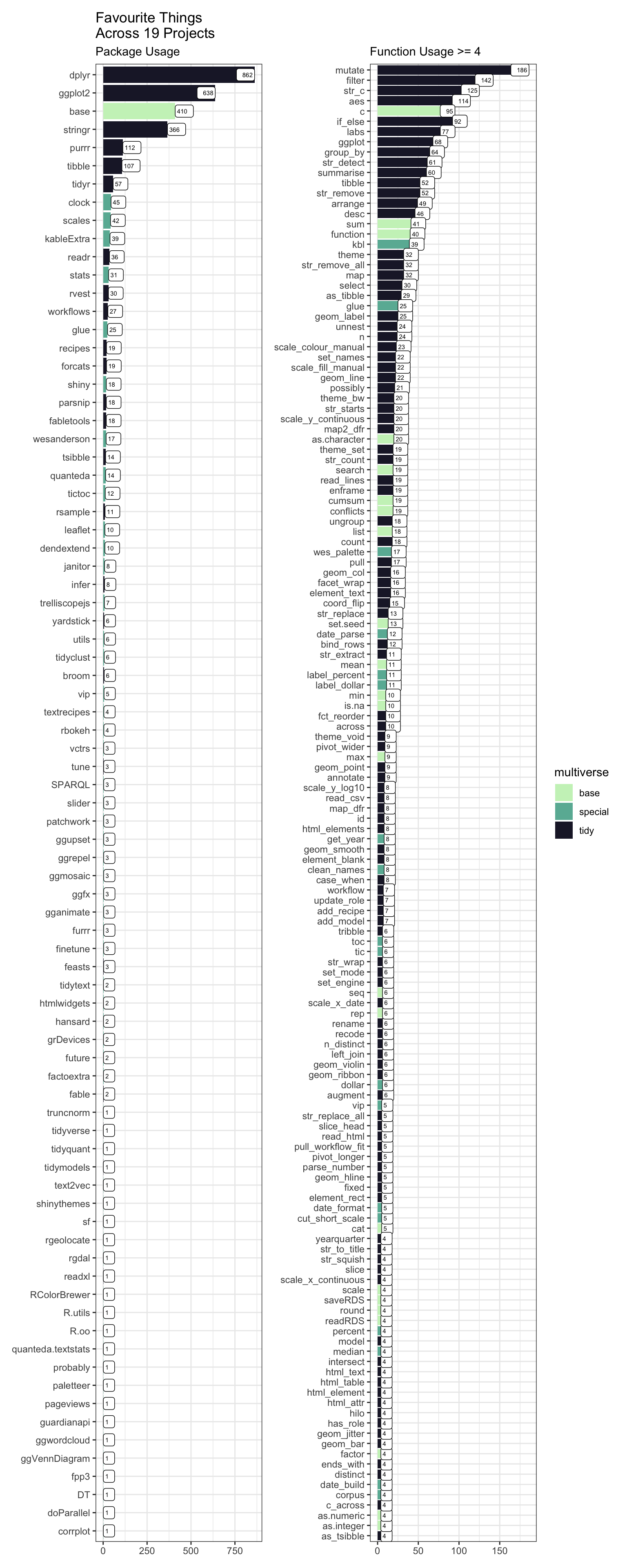
Clearly dplyr reigns supreme driven by mutate and filter.

p1 <- packfun_df |>
  filter(name == "package") |> 
  ggplot(aes(fct_reorder(packfun, n), n, fill = multiverse)) +
  geom_col(show.legend = FALSE) +
  coord_flip() +
  geom_label(aes(label = n), hjust = "inward", size = 2, fill = "white") +
  scale_fill_manual(values = cols[c(1, 2, 4)]) +
  labs(
    title = glue("Favourite Things\nAcross {n_url} Projects"),
    subtitle = "Package Usage",
    x = NULL, y = NULL
  )

p2 <- packfun_df |>
  filter(name == "function", n >= 4) |> 
  ggplot(aes(fct_reorder(packfun, n), n, fill = multiverse)) +
  geom_col() +
  coord_flip() +
  geom_label(aes(label = n), hjust = "inward", size = 2, fill = "white") +
  scale_fill_manual(values = cols[c(1, 2, 4)]) +
  labs(x = NULL, y = NULL, 
       subtitle = "Function Usage >= 4")

p1 + p2

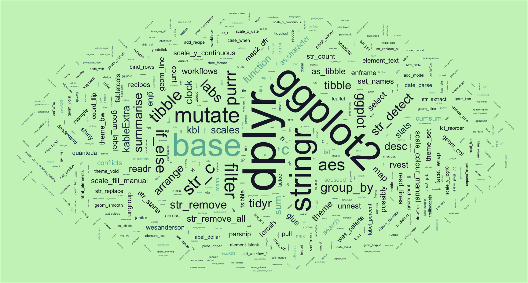
I’d also like a word cloud generated as the new featured image for this project.

set.seed = 123

packfun_df |>
  mutate(angle = 45 * sample(-2:2, n(), 
                             replace = TRUE, 
                             prob = c(1, 1, 4, 1, 1))) |>
  ggplot(aes(
    label = packfun,
    size = n,
    colour = multiverse,
    angle = angle
  )) +
  geom_text_wordcloud(
    eccentricity = 1,
    seed = 789
  ) +
  scale_size_area(max_size = 20) +
  scale_colour_manual(values = cols[c(2, 3, 4)]) +
  theme_void() +
  theme(plot.background = element_rect(fill = cols[1]))

R Toolbox

A little bit circular, but I might as well include this code too in my “favourite things”.

Package	Function
base	as.character[1]; as.integer[1]; c[5]; conflicts[1]; cumsum[1]; function[2]; sample[1]; search[1]; sum[1]; unique[1]
dplyr	filter[7]; arrange[3]; bind_rows[1]; case_when[1]; coalesce[1]; count[4]; desc[3]; group_by[2]; if_else[3]; mutate[10]; n_distinct[1]; pull[1]; select[1]; summarise[1]; transmute[1]
forcats	fct_reorder[2]; fct_rev[2]
fpp3	fpp3_packages[1]
ggplot2	aes[7]; annotate[1]; coord_flip[2]; element_rect[1]; geom_col[3]; geom_label[3]; ggplot[4]; labs[2]; scale_colour_manual[1]; scale_fill_manual[3]; scale_size_area[1]; theme[2]; theme_bw[1]; theme_set[1]; theme_void[2]
ggwordcloud	geom_text_wordcloud[1]
glue	glue[1]
janitor	clean_names[1]
kableExtra	kbl[1]
paletteer	paletteer_c[1]
purrr	map[1]; map_dfr[1]; map2_dfr[1]; possibly[1]; set_names[1]
readr	read_lines[1]
rvest	html_attr[1]; html_elements[2]; html_table[1]; read_html[2]
stringr	str_c[6]; str_count[1]; str_detect[2]; str_remove[4]; str_remove_all[1]; str_squish[1]; str_starts[1]
tibble	as_tibble[2]; tibble[3]; enframe[1]
tidymodels	tidymodels_packages[1]
tidyr	drop_na[1]; separate[1]; separate_rows[1]; unnest[1]
tidyverse	tidyverse_packages[1]

Posted:: July 26, 2020

Updated:: October 8, 2022

Length:: 4 minute read, 722 words

Categories:: R

Tags:: web scraping quarto

See Also:: Plots Thicken; Set Operations