House Sales
By Carl Goodwin in R
December 17, 2017
Various events have impacted house sales in London. There has been a series of increases in stamp duty and the impact of the financial crisis. More recently Brexit and the consequences of Covid-19.
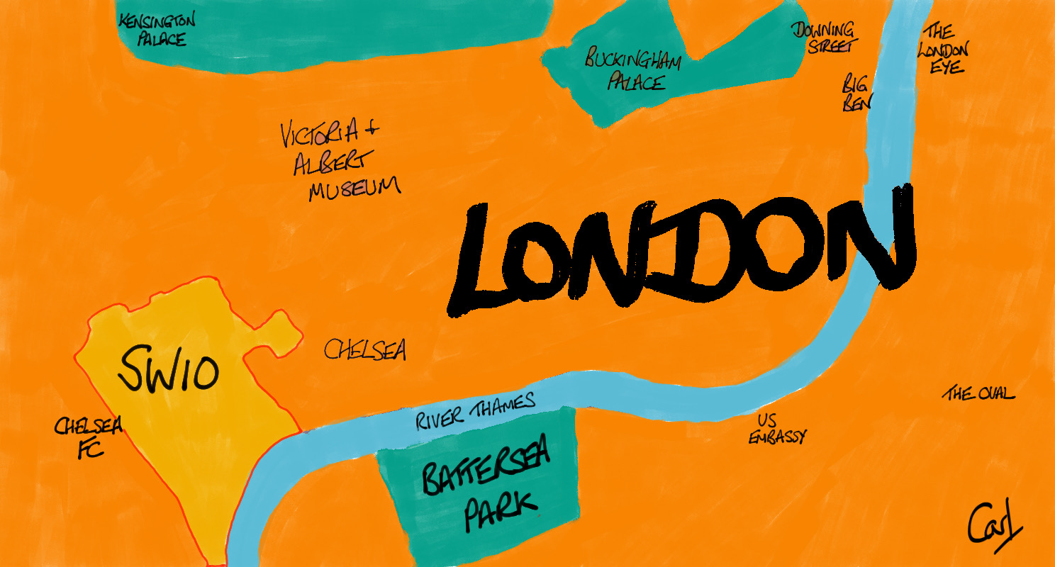
How is London postal area SW10 coping with all this?
library(tidyverse)
library(scales, exclude = "date_format")
library(SPARQL)
library(clock)
library(wesanderson)
library(glue)
library(vctrs)
library(tsibble)
library(patchwork)
library(ggmosaic)
library(kableExtra)
theme_set(theme_bw())

(cols <- wes_palette(name = "Darjeeling1"))

House prices paid data are provided by HM Land Registry Open Data.
endpoint <- "https://landregistry.data.gov.uk/landregistry/query"

query <- 'PREFIX  text: <http://jena.apache.org/text#>
PREFIX  ppd:  <http://landregistry.data.gov.uk/def/ppi/>
PREFIX  lrcommon: <http://landregistry.data.gov.uk/def/common/>

SELECT  ?item ?ppd_propertyAddress ?ppd_hasTransaction ?ppd_pricePaid ?ppd_transactionCategory ?ppd_transactionDate ?ppd_transactionId ?ppd_estateType ?ppd_newBuild ?ppd_propertyAddressCounty ?ppd_propertyAddressDistrict ?ppd_propertyAddressLocality ?ppd_propertyAddressPaon ?ppd_propertyAddressPostcode ?ppd_propertyAddressSaon ?ppd_propertyAddressStreet ?ppd_propertyAddressTown ?ppd_propertyType ?ppd_recordStatus

WHERE
{ ?ppd_propertyAddress text:query _:b0 .
  _:b0 <http://www.w3.org/1999/02/22-rdf-syntax-ns#first> lrcommon:postcode .
  _:b0 <http://www.w3.org/1999/02/22-rdf-syntax-ns#rest> _:b1 .
  _:b1 <http://www.w3.org/1999/02/22-rdf-syntax-ns#first> "( SW10 )" .
  _:b1 <http://www.w3.org/1999/02/22-rdf-syntax-ns#rest> _:b2 .
  _:b2 <http://www.w3.org/1999/02/22-rdf-syntax-ns#first> 3000000 .
  _:b2 <http://www.w3.org/1999/02/22-rdf-syntax-ns#rest> <http://www.w3.org/1999/02/22-rdf-syntax-ns#nil> .
  ?item ppd:propertyAddress ?ppd_propertyAddress .
  ?item ppd:hasTransaction ?ppd_hasTransaction .
  ?item ppd:pricePaid ?ppd_pricePaid .
  ?item ppd:transactionCategory ?ppd_transactionCategory .
  ?item ppd:transactionDate ?ppd_transactionDate .
  ?item ppd:transactionId ?ppd_transactionId

  OPTIONAL { ?item ppd:estateType ?ppd_estateType }
  OPTIONAL { ?item ppd:newBuild ?ppd_newBuild }
  OPTIONAL { ?ppd_propertyAddress lrcommon:county ?ppd_propertyAddressCounty }
  OPTIONAL { ?ppd_propertyAddress lrcommon:district ?ppd_propertyAddressDistrict }
  OPTIONAL { ?ppd_propertyAddress lrcommon:locality ?ppd_propertyAddressLocality }
  OPTIONAL { ?ppd_propertyAddress lrcommon:paon ?ppd_propertyAddressPaon }
  OPTIONAL { ?ppd_propertyAddress lrcommon:postcode ?ppd_propertyAddressPostcode }
  OPTIONAL { ?ppd_propertyAddress lrcommon:saon ?ppd_propertyAddressSaon }
  OPTIONAL { ?ppd_propertyAddress lrcommon:street ?ppd_propertyAddressStreet }
  OPTIONAL { ?ppd_propertyAddress lrcommon:town ?ppd_propertyAddressTown }
  OPTIONAL { ?item ppd:propertyType ?ppd_propertyType }
  OPTIONAL { ?item ppd:recordStatus ?ppd_recordStatus }
}'

data_list <- SPARQL(endpoint, query)
The focus is on the standard price paid.
data_tidy <- data_list$results |>
  as_tibble() |>
  mutate(
    date = new_datetime(ppd_transactionDate) |> as_date(),
    amount = ppd_pricePaid,
    prop_type = str_extract(ppd_propertyType, "(?<=common/)[\\w]+"),
    est_type = str_extract(ppd_estateType, "(?<=common/)[\\w]+"),
    cat = str_remove(ppd_transactionCategory, "<http://landregistry.data.gov.uk/def/ppi/"),
    prop_type = recode(prop_type, otherPropertyType = "Other")
  ) |>
  filter(str_detect(cat, "standard"))
A Telegraph article entitled Timeline: 20 years of stamp duty increases for home buyers pinpoints many of the key event dates.
events <- tribble(
  ~date, ~change,
  "96-07-31", "Stamp Duty £250k (1.5%) £500k (2%)",
  "98-03-31", "£250k (2%) £500k (3%)",
  "99-03-31", "£250k (2.5%) £500k (3.5%)",
  "00-03-31", "£250k (3%) £500k (4%)",
  "11-04-30", "£250k (3%) £500k (4%) £1m (5%)",
  "12-03-31", "£250k (3%) £500k (4%) £1m (5%) £2m (7%)",
  "14-12-31", "£250k (5%) £925k (10%) 1.5m (12%)",
  "07-08-09", "Financial Crisis",
  "16-06-23", "Brexit Vote",
  "20-03-23", "Covid-19 Lockdown"
) |>
  mutate(date = date_parse(date, format = "%y-%m-%d"))

events |>
  kbl(col.names = c("Date", "Event"))
| Date | Event |
|---|---|
| 1996-07-31 | Stamp Duty £250k (1.5%) £500k (2%) |
| 1998-03-31 | £250k (2%) £500k (3%) |
| 1999-03-31 | £250k (2.5%) £500k (3.5%) |
| 2000-03-31 | £250k (3%) £500k (4%) |
| 2011-04-30 | £250k (3%) £500k (4%) £1m (5%) |
| 2012-03-31 | £250k (3%) £500k (4%) £1m (5%) £2m (7%) |
| 2014-12-31 | £250k (5%) £925k (10%) 1.5m (12%) |
| 2007-08-09 | Financial Crisis |
| 2016-06-23 | Brexit Vote |
| 2020-03-23 | Covid-19 Lockdown |
Visually, it appears that the financial crisis had a big impact on sales volume, with the Brexit vote sucking much of the remaining oxygen out of the market. Stamp duty increases in between probably slowed any intermediate recovery.
to_date <- data_tidy |> summarise(max(date)) |> pull() |> date_format(format = "%b %d, %Y")

data_tidy |>
  ggplot(aes(date, amount, colour = est_type)) +
  geom_point(alpha = 0.2, size = 0.7, show.legend = FALSE) +
  geom_smooth(se = FALSE, aes(linetype = est_type), size = 1.2) +
  labs(
    title = "SW10 Standard House Prices",
    subtitle = glue("Prices Paid to {to_date} (Prices > £5m Not Shown)"
    ),
    x = NULL,
    y = NULL,
    colour = "Type", linetype = "Type",
    caption = "Source: HM Land Registry"
  ) +
  geom_vline(xintercept = events$date, size = 0.5, lty = 2, alpha = 0.4) +
  annotate("text", events$date, 5000000,
    angle = 90,
    label = events$change, vjust = 1.4, hjust = 1, size = 3, fontface = 2
  ) +
  coord_cartesian(ylim = c(0, 5000000)) +
  scale_colour_manual(values = cols[c(2, 3)]) +
  scale_x_date(date_breaks = "2 years", date_labels = "%Y") +
  scale_y_continuous(labels = label_dollar(accuracy = 0.1, prefix = "£",
                                           scale_cut = cut_short_scale()))

An alternative way of looking at this is by median quarterly prices (with upper and lower quartiles), supplemented by sales volumes.
qtr_start <- date_today("Europe/London") |>
  lubridate::floor_date("quarter")

data_qtile <-
  data_tidy |>
  filter(date < qtr_start) |>
  mutate(yr_qtr = yearquarter(date)) |>
  group_by(yr_qtr) |>
  summarise(price = quantile(amount, c(0.25, 0.5, 0.75)),
            quantile = c("lower", "median", "upper") |> factor(),
            n = n()) |>
  ungroup() |>
  pivot_wider(names_from = quantile, values_from = price)

last <- data_qtile |> summarise(max(yr_qtr)) |> pull()
first <- data_qtile |> summarise(min(yr_qtr)) |> pull()

p1 <- data_qtile |>
  ggplot(aes(yr_qtr, median)) +
  geom_ribbon(aes(ymin = lower, ymax = upper), fill = cols[5]) +
  geom_line(colour = "white") +
  geom_hline(yintercept = 1000000, linetype = "dashed") +
  annotate("text", x = 17700, y = 300000, label = "Covid-19\nLockdown", size = 3) +
  scale_x_yearquarter(date_breaks = "2 years") +
  scale_y_log10(labels = label_dollar(prefix = "£", scale_cut = cut_short_scale())) +
  labs(title = glue("Median Quarterly SW10 Property Prices ({first} to {last})"),
       subtitle = "With Upper / Lower Price Quartiles & Sales Volume",
       x = NULL, y = "Price (Log10 Scale)") +
  theme(axis.text.x = element_blank())

p2 <- data_qtile |>
  ggplot(aes(yr_qtr, n)) +
  geom_line() +
  annotate("text", x = 14100, y = 180, label = "Financial\nCrisis", size = 3) +
  annotate("text", x = 17100, y = 130, label = "Brexit\nVote", size = 3) +
  scale_x_yearquarter(date_breaks = "2 years") +
  labs(x = NULL, y = "Transactions",
       caption = "Source: HM Land Registry") +
  theme(axis.text.x = element_text(angle = 45, hjust = 1))

p1 / p2 + plot_layout(heights = c(2, 1))

The composition of SW10 reveals the postal area to be overwhelmingly dominated by leasehold flats.
trans <- data_tidy |> nrow()

data_tidy |>
  ggplot() +
  geom_mosaic(aes(product(prop_type, est_type), fill = prop_type),
              offset = 0.02, divider = mosaic("h")) +
  scale_fill_manual(values = cols[c(2:5)]) +
  labs(
    title = "SW10 Transactions by Estate & Property Types",
    subtitle = glue("{comma(trans)} Transactions to {to_date}"),
    x = "", y = "", fill = "Property Type",
    caption = "Source: HM Land Registry"
  ) +
  theme_minimal()

Other blog posts on quantum jitter look at SW10 property from diffferent perspectives: Digging Deep considers the correlation between house sales and planning applications; and Bootstraps & Bandings uses a sample of recent house sales to infer whether property bands are as representative of property values today as they were three decades ago.
R Toolbox
Summarising below the packages and functions used in this post enables me to separately create a toolbox visualisation summarising the usage of packages and functions across all posts.
| Package | Function |
|---|---|
| base | c[5]; conflicts[1]; cumsum[1]; factor[1]; function[1]; max[2]; min[1]; nrow[1]; search[1]; sum[1] |
| clock | as_date[1]; date_format[1]; date_parse[1]; date_today[1] |
| dplyr | filter[7]; arrange[2]; desc[2]; group_by[2]; if_else[3]; mutate[7]; n[2]; pull[3]; recode[1]; summarise[5]; ungroup[1] |
| ggmosaic | geom_mosaic[1]; mosaic[1]; product[1] |
| ggplot2 | aes[6]; annotate[4]; coord_cartesian[1]; element_blank[1]; element_text[1]; geom_hline[1]; geom_line[2]; geom_point[1]; geom_ribbon[1]; geom_smooth[1]; geom_vline[1]; ggplot[4]; labs[4]; Scale[1]; scale_colour_manual[1]; scale_fill_manual[1]; scale_x_date[1]; scale_y_continuous[1]; scale_y_log10[1]; theme[2]; theme_bw[1]; theme_minimal[1]; theme_set[1] |
| glue | glue[3] |
| kableExtra | kbl[2] |
| patchwork | plot_layout[1] |
| purrr | map[1]; map2_dfr[1]; possibly[1]; set_names[1] |
| readr | read_lines[1] |
| scales | comma[1]; cut_short_scale[2]; label_dollar[2] |
| SPARQL | SPARQL[1] |
| stats | median[1]; quantile[1] |
| stringr | str_c[5]; str_count[1]; str_detect[3]; str_extract[2]; str_remove[3]; str_remove_all[1]; str_starts[1] |
| tibble | as_tibble[2]; tibble[2]; tribble[2]; enframe[1] |
| tidyr | pivot_wider[1]; unnest[1] |
| tsibble | scale_x_yearquarter[2]; yearquarter[1] |
| vctrs | new_datetime[1] |
| wesanderson | wes_palette[1] |
- Posted:
- December 17, 2017
- Updated:
- April 21, 2022
- Length:
- 6 minute read, 1119 words
- Categories:
- R
- See Also: